PIVOT TABLES

Pivot table is a statistics tool in MS Excel that summarizes and reorganizes selected columns and rows of data in a spreadsheet or database table to obtain a desired report. The tool does not actually change the spreadsheet or database itself, it simply “pivots” or turns the data to view it from different perspectives.
With pivot tables, you can analyze data to reveal patterns and trends!
How Pivot Tables Work
When users create a pivot table, there are four main components:
- Columns- When a field is chosen for the column area, only the unique values of the field are listed across the top.
- Rows- When a field is chosen for the row area, it populates as the first column. Similar to the columns, all row labels are unique values, and duplicates are removed.
- Values- Each value is kept in a pivot table cell and displays the summarized information. The most common values are sum, average, minimum, and maximum.
- Filters- Filters apply a calculation or restriction to the entire table.
About Pivot Tables
A Pivot Table is an interactive way to quickly summarize large amounts of data. You can use a Pivot Table to analyze numerical data in detail and answer unanticipated questions about your data. A Pivot Table is specially designed for:
- Querying large amounts of data in many user-friendly ways.
- Subtotaling and aggregating numeric data, summarizing data by categories and subcategories and creating custom calculations and formulas.
- Expanding and collapsing levels of data to focus your results and drilling down to details from the summary data for areas of interest to you.
- Moving rows to columns or columns to rows (or “pivoting”) to see different summaries of the source data.
- Filtering, sorting, grouping, and conditionally formatting the most useful and interesting subset of data enables you to focus on just the information you want.
- Presenting concise, attractive, and annotated online or printed reports.
How to Create a Pivot Table in Excel: A Step-by-Step Tutorial
To create a Pivot Table in Excel, execute the following steps:
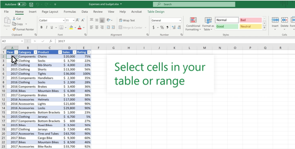
- Select cells in your table or range.
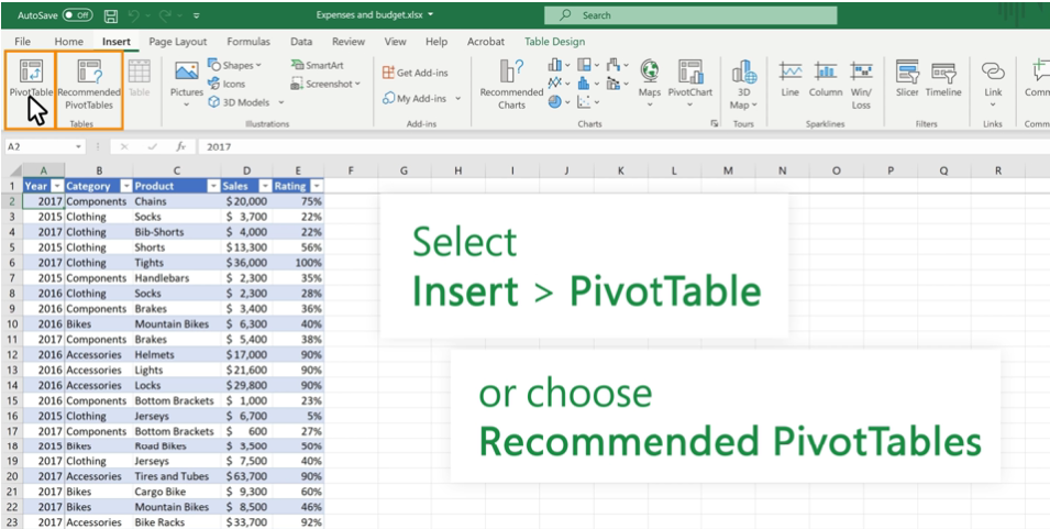
2. Select Insert>PivotTable or choose Recommended PivotTables.
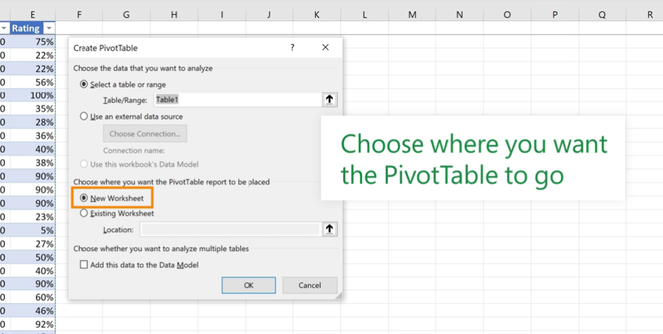
3. After clicking PivotTable, choose where you want the PivotTable to go, then click OK.
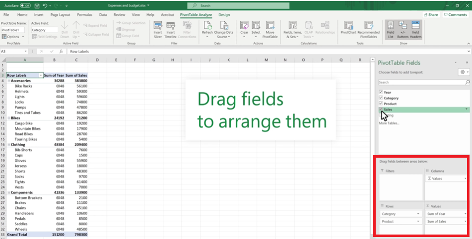
4. PivotTable Fields: Year, Category, Product, Sales, Rating. Add the fields you want.
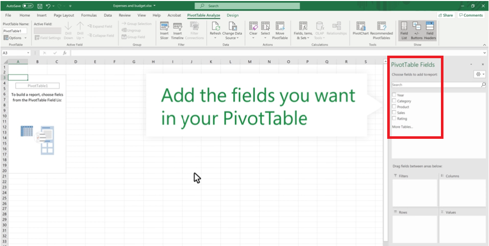
5. Drag the fields to new areas and see how you want data to be arranged.
Note: This process goes for non-iOS software.